Fitting lossless rainbow tables on a 4 TB disk and cracking NetNTLMv1 with WebGPU and ntlmrain.
Google’s release of the NetNTLMv1 rainbow tables made it much more practical to recover an NT hash from a NetNTLMv1 response captured with the fixed challenge 1122334455667788, further reducing the needed compute power.
NetNTLMv1 cracking is a problem I’ve kept returning to over the past several years. The recent table release prompted me to explore whether the process could be made cheaper, faster and easier to run. This post describes the result: a compact indexed table format, a WebGPU browser client and a native command-line tool.
Highlights
This post explains a new ntlmrain rainbow table layout. We are publicly releasing a browser tool and command-line client together with the optimized tables.
- Compressed rainbow tables: The original rainbow tables have been reworked for fast lookup from a 4 TB (3.64 TiB) consumer disk. This is a lossless compression that introduces a global index for faster lookups. On SSD this allows us to perform table lookups in under a minute.
- NTLMRain web lookup: A browser interface that uses WebGPU to recover the NT hash from a NetNTLMv1 response. Endpoint precomputation and candidate verification run locally on the user’s GPU. Table lookup is performed remotely. Neither the NetNTLMv1 response nor the cracked hash leave the browser (endpoints/candidates are exchanged with the remote service).
- Table lookup service: We’re hosting a central lookup service. The browser sends its derived endpoint file to this service and receives candidate chains, so you do not need to download or store the 4 TB table collection yourself.
- CLI tool: We are releasing a standalone command-line client
ntlmrain. It can use the hosted lookup service or search a locally stored copy of the tables. It supports both WebGPU and native CPU compute paths (which is surprisingly fast).
Check it out:
Context and relevance
NetNTLMv1 is (luckily) becoming less relevant. However, from time to time, we still come across NetNTLMv1-enabled systems. If that happens on a domain controller, you can compromise the domain by recovering the NT hash of the DC. Several blog posts explain this approach, such as the article by Yeray Martin on NTLMv1 DC Rainbow Tables: Domain Compromise.
Using the tooling we release today, we hope to further lower the barrier by reducing the cost, time and effort required to crack these responses.
Even on systems with Credential Guard enabled, NetNTLMv1 has also become relevant again. The DumpGuard tooling by Valdemar Carøe allows to obtain the NetNTLMv1 response for users on the system.
However, Microsoft describes the NetNTLMv1 protocol as removed from Windows 11 24H2+ and Windows Server 2025. That does not mean every NetNTLMv1 cryptographic primitive disappeared with it. Windows still contains interfaces that can generate NetNTLMv1-derived responses for certain scenarios.
We expect that, despite this enforcement, NetNTLMv1 cracking will likely remain relevant in several scenarios. For example, when encountering outdated systems and environments, printers, NAS storages, and Wi-Fi/VPN/Ethernet using MS-CHAPv2 auth. Administrators can also still manually override the BlockNtlmv1SSO setting back to auditing mode.
Recap of NetNTLMv1 cracking
A NetNTLMv1 response consists of three DES ciphertext blocks. The client derives their keys from the 16-byte NT hash:
- DES1 uses the first seven bytes;
- DES2 uses the next seven bytes; and
- DES3 uses the final two bytes followed by zero padding.
See the format explanation at Shuck.sh, which provides a useful visual breakdown of the challenge, DES keys and ciphertext components.
The tables released by Google target the 56-bit DES key space for the fixed challenge 1122334455667788. DES1 and DES2 use the table workflow. DES3 contains only 16 unknown bits and is recovered locally.
For each of the first two ciphertext blocks, recovery has three stages:
- Precompute: walk forward from the target ciphertext at every possible chain position, producing 881,688 endpoints.
- Lookup: find those endpoints in the table and return the matching chain starts. These are candidates, not confirmed keys.
- Verify: regenerate each candidate chain to the relevant position, reject collisions, and verify the recovered DES key against the complete 64-bit ciphertext.
The recent SpecterOps article Into The Rainbow: Google’s NTLMv1 Rainbow Tables Explained in a Bit Too Much Detail gives a useful walkthrough of these stages.
The collection contains 4096 source tables with 134,217,668 chains each: 549,755,568,128 chains in total. Every original .rt record occupies 16 bytes:
- 8-byte chain start + 8-byte chain endpoint = 16 bytes
- 549,755,568,128 × 16 = 8,796,089,090,048 bytes (8 TiB)
Optimizing table storage and lookups
Compressing the tables
Consumer disks typically advertise their storage in TB (10^12 bytes) rather than TiB (2^40 bytes). So if you buy an 8 TB disk, you will get 7.28 TiB and find out you actually needed a larger disk to store the 8 TiB tables. Since storage cost has increased dramatically, I was hoping we could store the data on a smaller disk, either an 8 TB, 6 TB, or even a 4 TB consumer disk.
The fields in the original rainbow tables are convenient to process, but they contain unused space.
As an example, while starts and endpoints consume 8 bytes (64 bits), a chain start needs only 39 bits because the complete collection contains fewer than 2^39 chains. An endpoint also only occupies a 56-bit DES space. This means we potentially only need 39+56 bits (95 bits) instead of 128 bits.
- 39-40 bits (rounded for easier storage) = 5-byte chain starts
- 56 bits = 7-byte chain ends
- 549,755,568,128 × 12 = 6,597,066,817,536 bytes
Even without compression, this reduces each record from 16 to 12 bytes, and is a good first step towards optimizing the storage. Similar popular optimizations already exist of course. Beyond the uncompressed RT format for rainbow tables, there are also the RTC (Compact) and RTI/RTI2 (Indexed) formats, which already dramatically reduce the storage requirements and lookup time.
- RTC compresses each table separately by storing size differences from estimated endpoints. The NetNTLMv1 tables have already been converted to the
RTCformat by duy-31, see NetNTLMv1-Perfect-Tables. This reduces the size down to 5.5 TB (5 TiB). - The RTI format further improved this with endpoint indexing. RTI2 allows configurable start and endpoint bit widths and stores a compact count for every endpoint prefix. Records still have one fixed size within a file though. The resulting tables would require around 4.4 TB. RTI2 keeps a separate index for every table part, so each lookup must consult up to 4096 indexes and read matching ranges from each.
Further storage optimizations have been suggested, such as by Avoine and Carpent.
For creating the compressed ntlmrain tables, we combine several of these techniques. While storage optimization is important, we also want lookup time to be as fast as possible. For this reason, we settled on a custom format.
These existing compact formats reduced the collection substantially. The public RTC conversion occupies about 5.5 TB, while RTI and practical RTI2 layouts remain above 4.4 TB once their indexes are included. That left an obvious target: could we make the entire table set fit on a single 4 TB consumer disk?
The ntlmrain table format
Endpoints become highly compressible after the 4096 original table parts are merged into a single globally sorted sequence. Since adjacent endpoint differences become smaller, they compress better.
The ntlmrain format uses three simple properties:
- 39-bit packed starts. Absolute start identifiers are packed next to each other instead of occupying 64 bits each.
- Endpoint differences. Globally sorted endpoints are stored as the difference from the preceding endpoint.
- Rice-16 coding. The average gap between endpoints is close to
2^17, which makes Rice coding with a 16-bit remainder a good fit. Try it out!
We named this compressed format GRTB. It doesn’t stand for anything, but if it needs an expansion, Giant Rainbow Table in a Bottle could describe it.
We are merely changing the representation of data. The format is lossless, retaining every endpoint and start point in the tables. The source tables can be reconstructed byte for byte from the converted collection.
| Field | Original | GRTB average |
|---|---|---|
| Chain start | 8 bytes | 4.875 bytes |
| Endpoint | 8 bytes | ~2.371 bytes |
| Total | 16 bytes | ~7.246 bytes |
The average record becomes approximately 7.246 bytes.

Figure 1: The global merge replaces fixed 64-bit fields with packed 39-bit starts and Rice-coded endpoint differences.
Adaptive 4 KiB pages
The encoded records are divided into fixed 4 KiB pages. This page size is intentional to align with common file system block sizes. In many cases, the OS will fetch 4 KiB of data regardless of how many bytes you want to actually read. If we wouldn’t do this, the record you’re querying could span several pages that need to be retrieved, causing extra disk reads.
As shown in the image above, each adaptive page contains a two-byte row count, Rice-16 endpoint differences and packed 39-bit starts. Records are added until the next one would exceed the page, at which point a new page begins.
Pages therefore hold a variable number of rows. The production collection has approximately 565 records per page on average. Adaptive filling brings the total storage size down to just below the storage threshold for a typical 4 TB (3.64 TiB) disk. A fixed number of records per page either wastes too much space or risks overflowing a page. Without it, the tables simply didn’t fit a 4 TB disk.
Total number of chains 549,755,568,128 x 7.246 bytes ≈ 3.98 TB.
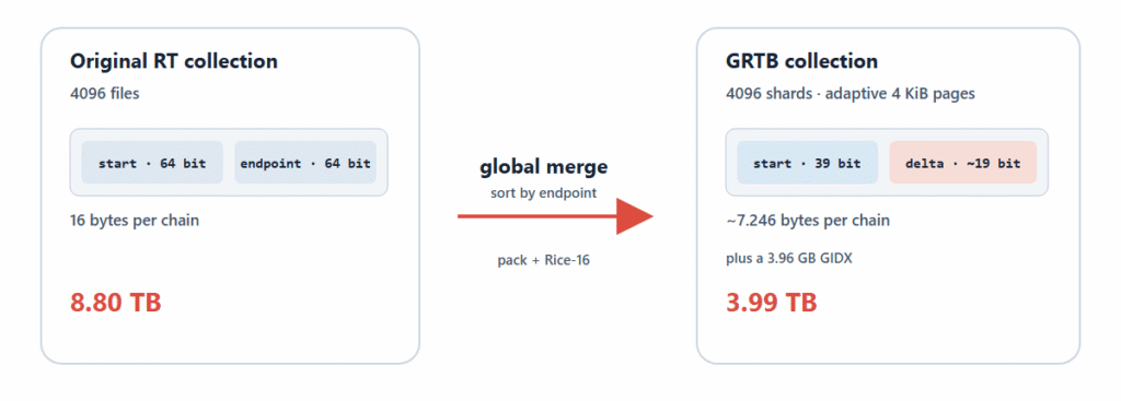
Figure 2: Adaptive pages combined with Rice-coding allow us to compress the data to just under 4TB
Searching efficiently
Since endpoints are globally sorted, we can now make a global lookup index (GIDX) that stores the endpoint boundary for each page. To resolve an endpoint, the reader searches the index, selects the relevant GRTB page, reads that 4 KiB page and decodes it. Lookup then returns every matching chain start.
In practice, for a full file of endpoints that we need to lookup, the lookup service first resolves all queries through the GIDX and then sorts the work by physical page.
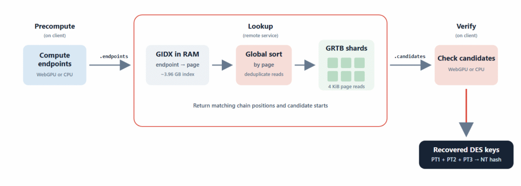
Figure 3: The service maps endpoints to pages and returns candidate starts.
Traditional RainbowCrack lookup operates on each sorted table separately, using binary search (or an index followed by a narrower binary search) to locate candidate endpoints. With thousands of table files, this still creates many independent searches and less efficient localized reads. GRTB/GIDX instead uses indexed and sorted page reads before accessing the shards.
Lookup performance
One DES half submits 881,688 endpoint queries. Let’s assume that a representative run selected 881,000 distinct GRTB pages: approximately 3.6 GB of logical 4 KiB reads scattered across the 4 TB disk. A complete NetNTLMv1 response requires two lookups (DES1 and DES2).
You can imagine that random-read latency and concurrency become important at that point.
| Storage | Two DES halves | Observed behavior |
|---|---|---|
| SSD – Virtual Netcup | ~1 minute | 30027 records/s |
| SSD – Azure Premium SSD v2, 60k IOPS, 1.5GBps | ~2 minutes | 16800 records/s |
| HDD – HGST Ultrastar He10 / DC HC510 | ~28 minutes | 1055 records/s |
Performance on NVMe storage would likely be faster, I would expect another significant speed increase for PCIe 4/5 NVMe on top of the Netcup speeds.
Download the tables
You can find/download the tables here: https://tables.ntlmrain.com/.
The resulting ntlmrain tables compress down to 3.99TB (3.63TiB) including the index.
| Data | Approximate size |
|---|---|
Original .rt collection | 8.80 TB / 8.00 TiB |
| GRTB shards | 3.98 TB / 3.62 TiB |
| GIDX index | 3.96 GB |
| GRTB+GIDX | 3.99 TB / 3.63 TiB |
The ntlmrain format reduces the original tables by 54.7%. The complete collection leaves only 12.6 GB of space before file system overhead. It fits, but only just.

If you plan on downloading the tables, filesystem choice and formatting options matter. Copying the files to a default-formatted volume and hoping for the best will likely not work out (speaking from experience). Using EXT4 or XFS with defaults may use up or reserve too much space for things like metadata.
I can’t personally vouch for these methods, but the following could work:
- XFS formatted with
reflink=0,rmapbt=0to disable metadata-heavy features:# Obviously confirm the correct device before doing this.mkfs.xfs -N -m reflink=0,rmapbt=0 /dev/DEVICE # dry runmkfs.xfs -f -L ntlmrain -m reflink=0,rmapbt=0 /dev/DEVICE
- EXT4 with largefile4 and no reserved-block allocation
- NTFS with compression/deduplication disabled
You can always fill the 4 TB disk as far as you can and host the few remaining tables or index on a separate (OS) volume. An SSD should be fast enough. Use NVMe if you want it even faster. I wouldn’t recommend a regular HDD as you will pay for seek latency (see the performance indications above).
Regardless of what you do, I recommend keeping the GIDX on fast storage and/or locking it into RAM.
Table lookup summary
The ntlmrain table format globally merges all endpoints, allowing one compact index to map each query directly to the relevant 4 KiB pages. Each page holds compressed records containing variable-width endpoint deltas. This makes it both smaller and much better suited to random batched lookup.
Note that these individual optimizations have been described before. However, I couldn’t find a pre-existing format that combined all these properties, allowed to perform fast lookups, and stayed within 4 TB. The downside is that it is very much tailored to NetNTLMv1 cracking at the moment rather than a generic reusable data format. Some of the concepts may port over however to other tables.
Precomputation and verification on WebGPU
Where table lookup is a storage workload, precompute and candidate verification are compute workloads.
Since our goal is to make NetNTLMv1 cracking more accessible and reducing compute, we also spent some time on making a portable WebGPU implementation with optimized shaders (with signifcant help of AI). Browsers can execute these through WebGPU, while a native client can use Rust’s wgpu implementation to run the same shaders through D3D12, Vulkan or Metal.
The original RainbowCrackalack implementation made use of OpenCL. Using OpenCL can definitely be faster because it can use vendor-specific features and perform lower-level operations. However, a WebGPU implementation is more portable.
RainbowCrackalack divides the work into OpenCL batches. A work item can still execute its entire remaining chain suffix in one kernel invocation. In the WebGPU port, we additionally slice the chain depth for better scheduling and occupancy. WebGPU enforces a strict 65535 workgroup dimension limit, and we need to avoid the browser’s WebGPU watchdog resets.
Two shader families are available:
- Compact: tiny shared memory footprint with little overhead. Compatible with almost every usable WebGPU adapter. However, every DES operation executes more integer instructions and separate table lookups. This shader is closer to the original OpenCL implementation.
- Expanded: uses fused S-box pairs and expanded key/permutation calculations. Less overall calculations, but requires more shared memory and potentially results in lower occupancy.
I played around with various other shader optimizations, memory strategies, and balancing additional fused S-box pairs, but in the end these were the only two that made a material difference on several tested (consumer) GPUs.
On a single RTX 4070Ti, the new shaders allow us to perform precomputation for a DES half in roughly 1 minute.
A CPU implementation was also made that uses SIMD/bitsliced DES that is decently fast. Further results in the performance overview below.
NTLMRain Web Lookup
The web lookup runs both GPU-heavy stages (precomputation, verification) locally in your browser as long as it exposes a WebGPU. The hosted service performs only the table lookup.
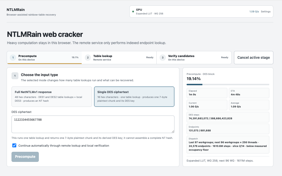
The browser accepts a 48-hex NetNTLMv1 response (or a 16-hex DES block) for the fixed 1122334455667788 challenge. For each DES half, the browser sends a ±7MB .endpoints file. It does not send the original NetNTLMv1 response, and the service never receives the recovered DES keys or resulting NT hash. It returns candidate chain starts, which the browser verifies locally.
However, this does not make a lookup fully anonymous. The endpoint set is deterministically derived from a DES target and could, with additional effort, serve as a fingerprint of that target. Treat it as such.
The hosted service keeps endpoint and candidate data only in memory for the short period needed to process and download a job. We do not log request bodies, endpoint sets, candidate results, NetNTLMv1 responses or recovered hashes. Requester IP addresses and request times are retained only as needed to operate the queue and enforce a fair-use policy.
Try out the NTLMRain Web Lookup.
NTLMRain command-line client
We are also releasing a native command-line tool for Windows, Linux and macOS. It supports GPU cracking but also has CPU fallback.
ntlmrain devicesntlmrain crack --netntlmv1 <48-hex-response>ntlmrain crack --des <16-hex-DES-block>ntlmrain precompute --netntlmv1 <48-hex-response>ntlmrain lookup <des1.endpoints> <des2.endpoints>ntlmrain verify --netntlmv1 <response> <des1.candidates> <des2.candidates>
By default, compute commands choose and tune a hardware WebGPU adapter: D3D12 on Windows, Vulkan on Linux and Metal on macOS. Multiple adapters can be listed and selected explicitly. Shader family, workgroup size and dispatch slicing can also be overridden.
If no eligible hardware GPU is available, a native CPU implementation will be used. The CPU path uses SIMD/bitsliced DES and the available logical processors.
The CLI can do lookups against the hosted lookup service or local lookup against the downloaded tables.
It supports running the precompute, lookup and verification stages individually, so you can resume between those.
Download the source and release packages on Outflank’s GitHub here: NTLMRain on GitHub.
Reference performance
The following empirical measurements cover a complete NetNTLMv1 response: two precompute passes, two table lookups and verification of both candidate sets. The listed totals are the observed complete runtimes, including lookup.
| Compute path | Device and configuration | Precompute | Verify | Total |
|---|---|---|---|---|
| WebGPU | NVIDIA GeForce RTX 4070 Ti, Compact, WG 64 | 1 min × 2 (6.5 G DES steps/s) | ~3 min | 7 min |
| WebGPU | NVIDIA GeForce RTX 2080 SUPER, Compact WG 64 | 3 min x 2 (2.1 G DES steps/s) | ~7 min | 14 min |
| WebGPU | Apple MacBook M1 Pro, Expanded, WG 1024 | 6 min × 2 (1.1 G DES steps/s) | ~10 min | 23 min |
| WebGPU | Intel Core Ultra 9 185H, Intel Arc, Compact, WG 512 | 20 min × 2 | ~20 min | 1 h 1 min |
| CPU | Intel Core Ultra 9 185H, 22 threads | 28 min × 2 | ~46 min | 1 h 43 min |
| CPU | AMD Ryzen 7 7800X3D, 16 threads | 14 min × 2 | ~30 min | 59 min |
They are real-life measurements that can vary. Candidate counts are variable per ciphertext, candidate verification is consequently variable too, and remote lookup can be affected by queue and transfer time. WebGPU performance also depends on the browser, driver and the selected configuration.
Defensive notes
The defensive conclusion remains straightforward: disable NetNTLMv1, prevent downgrade and coercion paths, and monitor where legacy authentication is still accepted. Google’s original release post includes concrete Group Policy and event-log guidance: Releasing Rainbow Tables to Accelerate Protocol Deprecation.
Acknowledgements
This work builds on a long line of research and implementation:
- Nic Losby led the effort to create and publish the NetNTLMv1 tables, documented in the January 2026 Google/Mandiant release post. Without that multi-year effort there would be no dataset to convert or use.
- Joe Testa created RainbowCrackalack, whose table algorithms and specialized NetNTLMv1 work formed an important technical foundation for this project.
- David Hulton built and operated the FPGA-backed DES cracking infrastructure. Moxie Marlinspike developed ChapCrack; together they presented the practical MS-CHAPv2 reduction and DES service at DEF CON 20. Hulton later documented the crack.sh service and API.
- Skyler Knecht documented the modern table workflow in the recent SpecterOps article.
- Philippe Oechslin introduced rainbow tables as the time-memory trade-off on which this work ultimately relies.
In particular thanks to:
- Dirk-jan Mollema for testing the clients and helping squash a steady supply of bugs.
- All the people who tolerated me shouting about rainbow tables out of nowhere from time to time.
We have released NTLMRain publicly on our GitHub. In addition, Outflank continually expands the tools and techniques available in Outflank Security Tooling (OST), a broad set of evasive tools that allow red team operators to safely and easily perform complex offensive tasks. We aim to expand the options available to red team operators through development of tools like our C2 implant and research into OS and EDR internals. Consider scheduling an expert-led demo to learn more about the diverse offerings in OST.